User Guide: Widgets & Tools

ROXAS AI provides a modular suite of widgets within the napari environment designed to take your wood cross-section images through the entire Quantitative Wood Anatomy (QWA) pipeline—from raw anatomical image to deep-learning segmentation, interactive manual curation, visual cross-dating, and measurement of anatomical traits.

Widgets are accessible via the napari Plugins > ROXAS AI menu and are numbered according to their typical execution sequence.

---

ROXAS AI Launcher & Startup

ROXAS AI provides a dedicated command-line entry point to launch napari pre-configured for wood anatomy workflows:

napari-roxas

What napari-roxas Does:

1. Installs Shortcuts Immediately: Registers global viewport navigation (WASD, Q/E) and widget group shortcuts (Ctrl+Shift+M/B/W) right from the start.
2. Docks the Manual Editing Group: Automatically opens the Manual Editing workflow container in the right sidebar, ready for immediate sample loading and inspection.

Launching via standard napari

You can also launch the application using standard napari. In this case, plugin shortcuts and duplicate prevention hooks activate automatically the moment any ROXAS AI widget or menu command is opened for the first time in that session.

---

Workflow Widget Groups & Dock Management

To eliminate sidebar clutter and streamline multi-step curation, ROXAS AI organizes individual tools into unified, scrollable Workflow Widget Groups:

flowchart LR
    subgraph Manual_Editing ["Manual Editing Group (Ctrl+Shift+M)"]
        direction TB
        M1["2/4 - Load Image(s)"] --> M2["3A - Detect Cells & Rings"]
        M2 --> M3["5 - Edit Cells"]
        M3 --> M4["6 - Edit Rings"]
        M4 --> M5["9A - Measure Cells & Rings"]
    end

    subgraph Batch_Operations ["Batch Operations Group (Ctrl+Shift+B)"]
        direction TB
        B1["1 - Prepare Project Images"] --> B2["3B - Batch Detect Cells & Rings"]
        B2 --> B3["9B - Batch Measure & Update"]
    end

    Cross["7 - Visual Crossdating"]
    Settings["ZZ - Settings"]
    ProjDir["0 - Define Project Directory"]

    ProjDir -.-> Manual_Editing & Batch_Operations
    Manual_Editing <--> Cross
    Settings -.-> Manual_Editing & Batch_Operations & Cross

1. Manual Editing Group (Ctrl+Shift+M)

Designed for interactive sample-by-sample analysis. It docks a single, scrollable container containing: - 2/4 - Load image(s) - 3A - Detect cells & rings (individual image) - 5 - Edit cells - 6 - Edit rings - 9A - Measure cells & rings (individual image)

2. Batch Operations Group (Ctrl+Shift+B)

Designed for high-throughput batch processing across entire project directories without loading individual images into the viewer. It docks: - 1 - Prepare project images for analysis - 3B - Batch detect cells & rings - 9B - Batch measure & update

3. Global Dock Management & Duplicate Prevention

• Close All Docks (Ctrl + Shift + W): Instantly closes all open dock widgets in the napari viewer.
• Duplicate Prevention: If you attempt to open an individual widget that is already loaded (either standalone or inside an active group), ROXAS AI displays a notification ('<Widget Name>' is already active in the sidebar.) and prevents duplicate dock instances.

For a complete reference of all available keyboard and mouse shortcuts, see the dedicated Shortcuts Reference.

Manual Editing Group (Ctrl+Shift+M)Batch Operations Group (Ctrl+Shift+B)

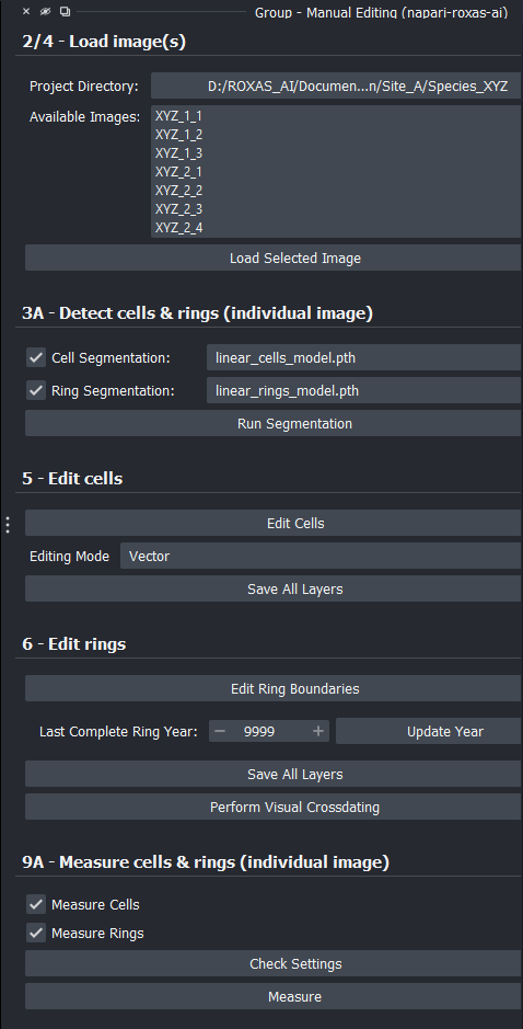
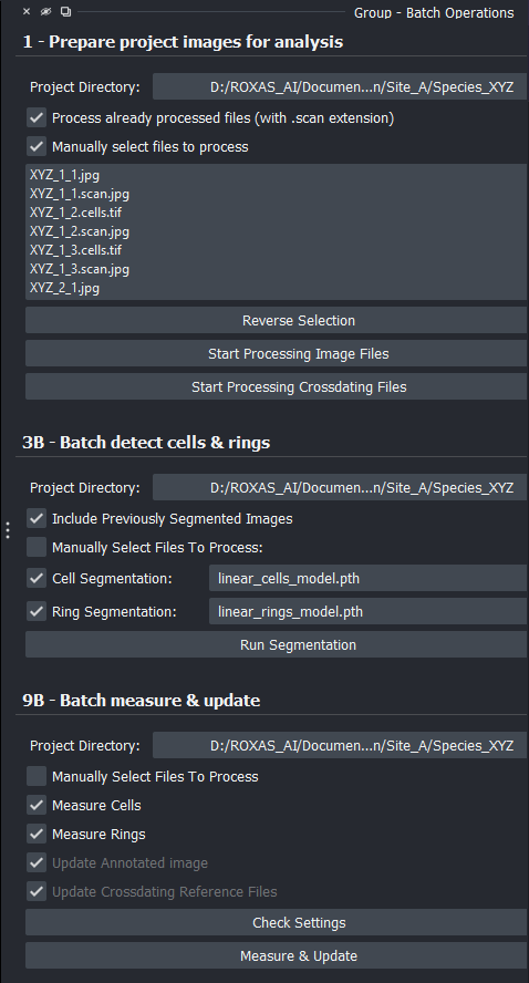
Figure 1: Workflow widget groups docked in the napari right sidebar: (A) Manual Editing Group and (B) Batch Operations Group.

---

Overview of Widgets & Tools

Widget Number & Name	Primary Purpose	Dedicated Shortcut (Scope)	Input	Output
0 - Define project directory	Set or change the active project working directory	—	Folder path	Global project path in settings.json
1 - Prepare project images for analysis	Standardize filenames, assign physical resolution, parse cross-dating files	Part of Batch Group (Ctrl+Shift+B)	Raw image files & reference series	<sample>.scan.<ext>, .metadata.json, rings_series.crossdating.txt
2/4 - Load image(s)	Load sample scans and associated cells/rings label layers	Part of Manual Group (Ctrl+Shift+M)	Prepared sample files	Image & Labels layers in viewer
3A - Detect cells & rings (individual image)	Run deep-learning segmentation on the currently active scan	Part of Manual Group (Ctrl+Shift+M)	Active scan image	.cells and .rings Labels layers
3B - Batch detect cells & rings	Run deep-learning segmentation across multiple samples in batch mode	Part of Batch Group (Ctrl+Shift+B)	Project directory / selected files	.cells.png, .rings.tif, .metadata.json
5 - Edit cells	Interactive curation of cell lumens (raster brush/eraser, vector polygons, lasso)	Ctrl+Wheel (Brush size), Ctrl+DblClick (Switch tool), Ctrl+Z (Undo) (Scope: 5 - Edit cells)	.cells layer	Refined .cells layer
6 - Edit rings	Interactive curation of tree-ring boundaries, nudging, wedging rings, re-runs	Ctrl+Arrows (1 px Nudge), Ctrl+Shift+Arrows (10 px Nudge), Ctrl+Z (Undo) (Scope: 6 - Edit rings)	.rings layer	Refined .rings layer & ring years
7 - Visual crossdating	Synchronize sample ring-width series against master reference chronologies	—	.rings layer & crossdating file	Synchronized ring years & reference plots
8 - Save cells & rings editing	Persist manual edits, masks, annotated scan images, and metadata to disk	—	Active ROXAS AI layers	.cells.png, .rings.tif, _annotated.jpg, .metadata.json
9A - Measure cells & rings (individual image)	Extract anatomical and tree-ring traits for active sample; generate CWT QA circles layer; update annotated image	Check Settings button (Scope: 9A - Measure cells & rings)	.cells & .rings layers	.cells_table.csv, .rings_table.csv, .cwt.json, _annotated.jpg
9B - Batch measure & update	Batch measurement extraction, .cwt.json export, annotated image generation, and reference plot updates	Part of Batch Group (Ctrl+Shift+B)	Project directory / selected files	Synchronized measurement tables, .cwt.json files, annotated images, and reference plots
ZZ - Settings	Preferences for hardware acceleration, visualization, tolerances, and measurements	Floating dialog via widgets or menu	User configuration	settings.json file

---

0 - Define Project Directory

The Define Project Directory widget configures the root folder where your sample images, metadata, and analysis tables reside.

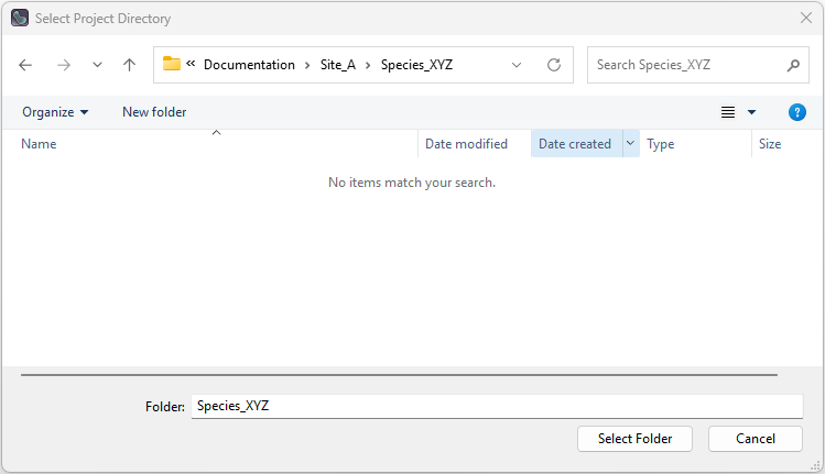
Figure 2: Project directory selection dialog.

How It Works

When triggered from the menu or from any widget directory button, it opens a system folder browser. Selecting a folder updates the project_directory entry in settings.json. All subsequent loading, saving, and batch processing widgets default to this directory. Note that the exact same directory selection functionality is also triggered whenever selecting the project directory directly from within widgets 1 - Prepare Project Images, 2/4 - Load Image(s), 3B - Batch Detect Cells & Rings, and 9B - Batch Measure & Update.

Inaccessible Directory Fallback

On multi-user systems, shared network drives, or when folders are moved or deleted, a previously saved directory path may become invalid or restricted:

• During startup and settings loading, ROXAS AI automatically validates read and execution permissions on the configured project_directory.
• If the directory cannot be accessed (e.g., PermissionError or non-existent path), ROXAS AI safely catches the error, notifies the user with a warning notification, and resets project_directory to "Not set" (None) rather than causing application crashes.

Key Controls

• Select Project Directory: Prompts the user to pick a folder. Upon confirmation, a notification displays the chosen path.

---

1 - Prepare Project Images for Analysis

The Prepare Project Images widget standardizes anatomical images and external cross-dating files into the structured file naming conventions and data structures required by ROXAS AI.

A: Main InterfaceB: Metadata Configuration DialogC: Cross-Dating Files Processing Dialog

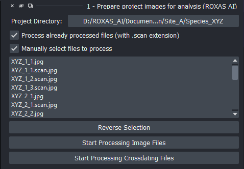
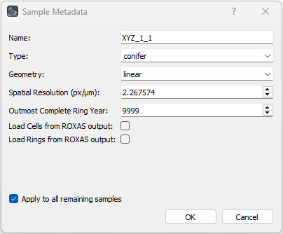
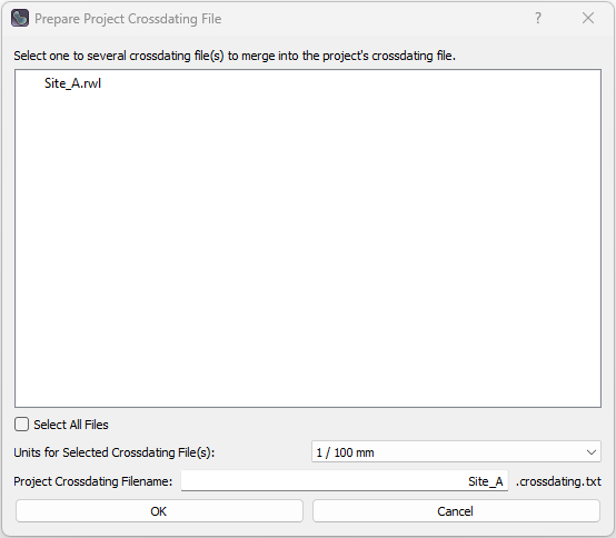
Figure 3: Prepare project images widget and interactive configuration dialogs: (A) Main preparation widget interface, (B) Interactive metadata configuration dialog, and (C) Cross-dating files compilation and unit scaling dialog.

How It Works

1. Scans the selected project directory (and subdirectories) for supported image formats (.jpg, .jpeg, .png, .tif, .tiff, .bmp, .jp2).
2. Opens an interactive Metadata Dialog for each sample to capture physical dimensions, spatial resolution (\(\mu\text{m}/\text{px}\)), sample type (e.g., conifer), measurement geometry (linear), and the outermost complete calendar year.
   • Apply to All Remaining Samples: The metadata prompt provides an Apply to all remaining samples checkbox. Enabling this applies the current metadata choices across all remaining samples in the batch without prompting again.
   • ROXAS Classic Migration / Output Loading: If a sample folder contains legacy ROXAS Classic output files, the dialog displays Load Cells from ROXAS output (which imports vessel segmentation masks from _Vessels.scl / .scl) and Load Rings from ROXAS output (which reconstructs ring boundaries, years, and label maps from _ringtraces.txt / _ringtraces.csv). This allows instant migration of existing ROXAS projects into ROXAS AI layers (.cells.png and .rings.tif) without re-running AI segmentation.
3. Automatically standardizes filenames to <sample>.scan.<ext> (safely handling cross-device moves and case-insensitive filesystem renames) and creates a synchronized <sample>.metadata.json.
4. Discovers and merges external cross-dating series (e.g., Tucson .rwl, .tuc, or tabular .txt/.csv files) into a unified reference file (rings_series.crossdating.txt, configured as [".crossdating", ".txt"] in settings.json) scaled to micrometers (\(\mu\text{m}\)).

Cross-Dating Text Files Processing

The Start Processing Crossdating Files action allows you to import and compile one or more external tree-ring width (TRW) measurement files or master reference chronologies into a single synchronized project cross-dating file.

Supported Input File Formats

The cross-dating parser automatically recognizes and parses several standard dendrochronological and tabular formats:

• Tabular Files (.csv, .tsv, .txt):

  • Delimiters: Auto-detected among tab (\t), comma (,), or semicolon (;).
  • Structure: Column-oriented or matrix tables where the first column or index contains the calendar year (YEAR), and additional columns contain tree-ring width series for individual trees, radii, or site chronologies.
  • Header handling: Automatically detects whether headers with series names exist or if the file contains pure numeric columns.

  Example Tabular Input (sample_series.txt or sample_series.csv, values in \(1/100\,\text{mm}\)):

  YEAR	Series01	Series02
  2018	142	165
  2019	118	130
  2020	155	148
  2021	98	112
  2022	125	135

• Tucson / Decadal Files (.rwl, .tuc):

  • Raw Tucson Decadal Format: Standard space-delimited format used by dendrochronology software (e.g., COFECHA, ARSTAN, TSAP-Win). Each line contains series_id, start_year, and up to 10 ring-width values followed by end-of-series sentinel markers (-9999, -999, 9999, or 999).
  • 8-Character Series Names: Series names of up to 8 characters are fully supported without collapsing into the YEAR column. The parsing algorithm detects when long series IDs abut the decade column and splits them smartly.
  • Tab-Delimited ("Doctored") Tucson Format: Tucson decadal files where fields are separated by tab characters. The parser identifies sentinel stop values and pivots the decadal entries into continuous annual time series.

  ATTENTION: Tucson/decadal files must be saved with the .rwl or .tuc extension. If an RWL file is saved or renamed with a .txt extension, it will not be processed correctly because the parser will attempt to read it as a standard tabular file rather than a decadal file.

  Example Tucson Input (site_chronology.rwl, values in \(1/100\,\text{mm}\)):

  Series01 2010   110  125  130  142  118  155   98  125  140  150
  Series01 2020   160  135  120 -9999
  

Unit Scaling Conversion

Because tree-ring measurement devices export widths in varying units, the selection dialog allows specifying the unit scale of the input files to convert all values into standard micrometers (\(\mu\text{m}\)):

Selected Unit Option	Multiplier Applied	Resulting Unit
1 / 1 mm	\(\times 1000.0\)	\(\mu\text{m}\)
1 / 10 mm	\(\times 100.0\)	\(\mu\text{m}\)
1 / 100 mm (default)	\(\times 10.0\)	\(\mu\text{m}\)
1 / 1000 mm	\(\times 1.0\)	\(\mu\text{m}\)
divide values by 10	\(\times 0.1\)	\(\mu\text{m}\)

Output File Structure & Merging Logic

The compiled series is saved in the project directory as <prefix><crossdating_file_extension> (by default rings_series.crossdating.txt, where file_extensions.crossdating_file_extension in settings.json is configured as [".crossdating", ".txt"], which concatenates to .crossdating.txt):

• Customizable Output Prefix: Users can customize the filename prefix in the dialog (defaulting to rings_series). This allows naming the cross-dating file after a site, project, or chronology acronym (e.g., TORN.PISY.crossdating.txt for a Pinus sylvestris chronology from the Torneträsk site).
• Updating and Merging Existing Files with Unit Scaling Logic: You can select multiple raw files alongside existing .crossdating.txt files to merge them into a single reference file or update an existing project cross-dating file.
  • Scaling suppression for existing .crossdating.txt files: Any selected file that is already a cross-dating output file (e.g., *.crossdating.txt or containing crossdating in its filename) is recognized as already converted to micrometers (\(\mu\text{m}\)). The chosen unit scaling multiplier is automatically suppressed (multiplier \(= 1.0\)) for these files.
  • Selective scaling for raw inputs: The selected unit scaling multiplier is applied only to newly added raw measurement files (.rwl, .tuc, standard .txt).
  • Priority handling: When merging, data from newly added raw files takes priority over older values in case of duplicate series and year combinations. This allows updating existing chronologies with new measurements while preserving previously imported data.
• Format & Delimiter: Tab-delimited plain text file (\t separator).
• Index (YEAR): The first column is named YEAR and contains unique calendar years spanning the complete chronological range across all imported series, sorted in ascending order.
• Series Columns: Each imported file/series forms its own named column header (derived from series IDs or column labels in the source files).
• Data Alignment & Missing Values: Ring widths are aligned by year across all series in micrometers (\(\mu\text{m}\)). Years not covered by a given series are left empty (NaN), allowing seamless integration of chronologies with differing time spans.

Example Output File (TORN.PISY.crossdating.txt, tab-delimited, values in \(\mu\text{m}\) after applying \(\times 10.0\) scaling to raw 1/100 mm files):

YEAR	Series01	Series02
2018	1420	1650
2019	1180	1300
2020	1550	1480
2021	980	1120
2022	1250	1350

Key Controls & Options

• Project Directory Button: Displays and allows switching the active project directory (triggering the same global project directory selection dialog).
• Process already processed files: When unchecked (default), skips files that already have the .scan extension.
• Manually select files to process: Expands a multi-selection list allowing selective processing of specific samples instead of the entire directory.
• Reverse Selection: Inverts the current file selection in the list.
• Automatic Filtering of ROXAS Output Files: The widget automatically ignores and excludes ROXAS AI output layers (.cells.*, .rings.*), annotated overviews (_annotated.jpg), cross-dating plots (_ReferenceSeries.jpg), and ROXAS Classic output files (_annotated_cells.jpg, _annotated_twin.jpg, _ReferenceSeries.gif, _Preview.jpg, etc.) from the candidate input list.
• Start Processing Image Files: Launches the preparation worker thread with a live progress bar.
• Start Processing Crossdating Files: Opens the cross-dating file selection, unit conversion, and custom filename prefix dialog to compile or update project reference series.

---

2/4 - Load Image(s)

The Samples Loading Widget loads prepared sample images (.scan), cell labels (.cells), and tree-ring labels (.rings) into napari with standardized colormaps, scaling, and navigation shortcuts.

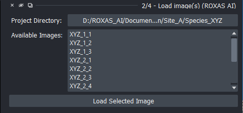
Figure 4: Samples loading widget interface.

How It Works

• Queries the project directory for prepared sample stems.
• Automatic Project Stem Path Repair: When opening a project directory that has been moved, renamed, or transferred from another computer/OS, ROXAS AI automatically repairs all sample_stem_path references in metadata to match the current filesystem location.
• Real-Time Directory Synchronization: Changes to the project directory are automatically synchronized and updated across all widgets in real-time.
• Single-Image Workflow Enforcement: Only one sample image can be loaded in the napari viewer at a time. Attempting to load another image prompts the user to first close the currently active image.
• Reads image layers along with their associated metadata (scale in \(\mu\text{m}/\text{px}\), sample stem paths, and ring year metadata) and automatically loads any available associated .rings and .cells layers.
• Automatic Ring Year Overlay Initialization: Background tracking monitors loaded layers so that calendar year labels (Rings Years text overlay) appear automatically in the viewer even if the ring editor widget is not docked.
• Automatic CWT Quality Assurance Circles: If a <sample>.cwt.json file is present in the sample folder and CWT visualization is enabled in settings (cwt_visualization.enabled = true), ROXAS AI automatically generates and displays the [<sample>] CWT Circles Shapes layer with interactive tooltips.
• Applies high-contrast colormaps (binary colormap for cells and distinct color cycling for rings).

Key Controls

• Project Directory Button: Displays and allows switching the active project directory (triggering the same global project directory selection dialog).
• Available Images List: Displays discovered sample scans in the current project directory. The list height dynamically adapts between 5 and 7 visible rows based on content. Double-clicking any sample entry immediately loads that image into the viewer along with its available associated rings and cells layers (identical to selecting the file and clicking Load Selected Image).
• Load Selected Image: Loads the currently selected sample file (along with available associated rings and cells layers) into the viewer.
• Progress Bar: Displays sample loading progress.

---

3A - Detect Cells & Rings (Individual Image)

The Single Sample Segmentation Widget performs automated deep-learning inference to identify tracheid cell lumens and annual tree-ring boundaries on the currently displayed image.

Automatic Background Model Downloads

Pre-trained neural network models (.pth / .pt weights) are downloaded automatically in the background if they are missing. Once downloaded, models are cached locally for all subsequent operations.

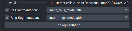
Figure 5: Single sample AI segmentation interface.

How It Works

• Runs neural network models (PyTorch / PyTorch Lightning / SMP architectures) locally on either GPU or CPU. For full architectural details and literature citations, see Deep-Learning Segmentation Models.
• Cells Detection: Predicts individual cell lumen instances using a U-Net architecture with a ResNet-50 backbone (Katzenmaier et al. 2023) and outputs a labeled mask layer (<sample>.cells).
• Rings Detection: Detects continuous tree-ring boundaries using an iterative regression formulation based on Katzenmaier et al. (2025), sorts boundaries from bark to pith, enforces boundary continuity across the sample width, and constructs labeled annual ring bands (<sample>.rings).
• Post-processes masks to eliminate edge artefacts (e.g., boundary-touching partial cells).

Files and Layers Saved

• In-Memory Layers Created / Updated: Adds or updates the <sample>.cells layer (Labels), <sample>.rings layer (Labels), and Rings Years text overlay layer in the active napari viewer.
• Annotated Overview Image: Automatically generates and saves the <sample>_annotated.jpg overview scan in the sample directory, overlaid with detected ring boundaries and calendar year labels (and optional semi-transparent cell overlays).
• Metadata: Updates <sample>.metadata.json with detected ring count (rings_count) and outermost complete year (rings_outmost_complete_year).
• Note on Label Files on Disk: The raw segmentation label rasters (.cells.png and .rings.tif) are held in memory as viewer layers ready for manual inspection/editing; they are persisted to disk when clicking Save All Layers (or via 8 - Save Cells & Rings Editing).

Key Controls & Options

• Cell Segmentation Checkbox & Model Dropdown: Checkbox to enable cell lumen detection, alongside a dropdown list to choose the trained cell model checkpoint (.pth). Unchecking disables cell detection and hides the model selection dropdown.
• Ring Segmentation Checkbox & Model Dropdown: Checkbox to enable tree-ring boundary detection, alongside a dropdown list to choose the trained ring model checkpoint (.pth). Unchecking disables ring detection and hides the model selection dropdown.
• Run Segmentation Button: Initiates the segmentation inference process in a non-blocking background worker thread. The button is automatically disabled if both segmentation options are unchecked.

---

3B - Batch Detect Cells & Rings

The Batch Sample Segmentation Widget executes AI detection across multiple samples in the background without needing to load each image into the viewer.

Automatic Background Model Downloads

If segmentation model weights are not present locally, they are automatically downloaded in the background when needed and cached for future runs.

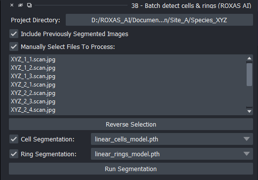
Figure 6: Batch sample segmentation interface.

How It Works

• Iterates over all discovered sample scans in the project directory.
• Applies the selected neural network models sequentially (see Deep-Learning Segmentation Models).
• Automatically saves segmentation masks (.cells.png and .rings.tif) directly to disk alongside updated .metadata.json files.

Files and Layers Saved

• Cell Masks (<sample>.cells.png): Saved directly to disk when cell segmentation is enabled.
• Ring Masks (<sample>.rings.tif): Saved directly to disk when ring segmentation is enabled.
• Annotated Overview Images (<sample>_annotated.jpg): Automatically created or updated on disk with ring boundaries and year labels when ring segmentation is run.
• Metadata (<sample>.metadata.json): Updated on disk with ring count (rings_count) and outermost complete year (rings_outmost_complete_year).

Key Controls

• Project Directory Selection: Choose the target folder containing prepared samples (triggering the same global project directory selection dialog).
• File Selection Mode: Toggle between Batch Process All Samples and handpicking subsets (Manually select files to process).
• Reverse Selection: Inverts current sample selections in the list.
• Segmentation Targets: Checkboxes for Segment Cells and Segment Rings.
• Model Dropdowns: Select weights for cell and ring models.
• Run Segmentation Button: Launches the batch worker with overall progress tracking.

---

5 - Edit Cells

The Cells Layer Editor Widget provides interactive manual editing tools to correct, split, merge, add, or erase cell lumen detections.

A: Startup (Idle)B: Vector ModeC: Lasso SelectionD: Raster Mode

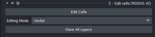
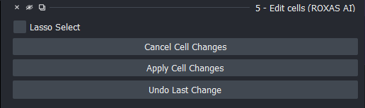
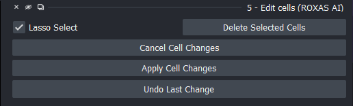
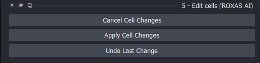
Figure 7: Cells layer editor widget in its four operational states: (A) Startup, (B) Vector editing active, (C) Vector editing with lasso selection enabled, and (D) Raster editing mode.

How It Works

• Mutual Editing Exclusion & Layer Guards: Temporarily transfers the active .cells layer into an editable working state (Cells Modification), while automatically hiding tree-ring layers (.rings and Rings Years) as well as CWT visualization circles ([<sample>] CWT Circles) to prevent visual clutter and accidental cross-layer modifications. Exiting editing mode automatically restores the previous visibility states.
• Supports two distinct editing paradigms:
  • Edit As Raster: Uses napari's native brush, paint bucket, and eraser tools directly on the label mask without geometric approximation.
    • Brush Size Adjustment: Adjust brush diameter smoothly between 1 and 100 px using Ctrl + Mouse Wheel (or trackpad scroll). Dimension slider scrolling is suspended during resizing.
    • Tool Switching: Quickly toggle between brush and eraser using Ctrl + Double-Click.
  • Edit As Vector: Converts cell outlines into editable polygon shapes for precise vertex editing, shape adjustment, and deletion (individual shapes can be selected directly using napari's shape selection tool or via freehand lasso loops).
• Lasso Selection & Union (OR) Behavior: In Vector editing mode, drawing lasso loops encloses cells. Multiple overlapping lasso polygons combine (union / OR logic) rather than toggling/canceling, allowing seamless regional selection.
• Undo Mechanism: Supports a 50-step history stack (Ctrl+Z or Undo Last Change button) that snapshots polygon coordinates and shape types in Vector mode, and triggers napari's label brush history in Raster mode.
• When applied, rasterizes vectors back to label masks, marks the .cells layer as modified (triggering unsaved change tracking), resets layer feature tables for fresh re-measurement, restores ring layer visibility, and preserves layer metadata.
• Customizable Tolerances & Colors: Polygon smoothing tolerances, line widths, and display colors can be customized in ZZ - Settings (see Technical Reference: Visualization Settings).

Files and Layers Saved

• In-Memory Modifications: Changes made using Vector or Raster tools are committed to the in-memory <sample>.cells layer upon clicking Apply Cell Changes.
• Saving to Disk: Clicking Save All Layers (or using 8 - Save Cells & Rings Editing) writes the updated <sample>.cells.png raster directly to disk and updates <sample>.metadata.json. Manual saving does not redraw <sample>_annotated.jpg (keeping saves fast); the annotated image is automatically updated at major workflow checkpoints (segmentation, year updates, cross-dating, measurements).

Key Controls & Options

• Editing Mode: Switch between Vector and Raster editing modes.
• Edit Cells: Enters editing mode, hides ring layers, and creates the working canvas (Cells Modification).
• Lasso Select: Checkbox (available during Vector editing) that activates a yellow Lasso Selection shapes layer for freehand polygon area selection.
• Delete Selected Cells: Deletes all cell polygons that intersect or touch the drawn lasso area, or those selected directly with the shape selection tool (can also be triggered using the Delete or Backspace key).
• Undo Last Change: Reverts the most recent edit (brush/eraser stroke, shape edit or lasso deletion) made during the active editing session (also available with Ctrl+Z).
• Apply Cell Changes: Commits edits, updates the .cells layer, restores layer visibility, and exits editing mode.
• Cancel Cell Changes: Discards pending modifications, removes the working layer, restores original layer visibility, and exits editing mode.
• Save All Layers: Persists all modified sample layers, metadata, and the annotated overview image directly to disk (see 8 - Save Cells & Rings Editing).

Dedicated Shortcuts

For a complete summary of all shortcuts across the application, see the Shortcuts Reference.

Action	Dedicated Shortcut	Scope
Adjust Brush Size	Ctrl + Mouse Wheel (macOS: Cmd + Wheel)	Active in 5 - Edit cells (Raster Mode)
Switch Brush / Eraser	Ctrl + Double-Click (macOS: Cmd + Double-Click)	Active in 5 - Edit cells (Raster Mode)
Delete Lasso Selection	Delete or Backspace	Active in 5 - Edit cells (Vector Mode)
Undo Last Change	Ctrl + Z	Active in 5 - Edit cells

---

6 - Edit Rings

The Rings Layer Editor Widget enables precise curation of annual tree-ring boundaries, outermost year re-numbering, fine nudging, handling of wedging rings, and targeted model-assisted re-detection.

Automatic Background Model Downloads

Opening this widget checks for missing ring segmentation model weights (required for the Rerun Ring Segmentation feature) and downloads them automatically in the background without blocking the interface. Once downloaded, models are cached locally for subsequent use.

A: Startup (Idle)B: Vector Boundary EditingC: Lasso Vertex DeletionD: Rerun Model from Year Workflow

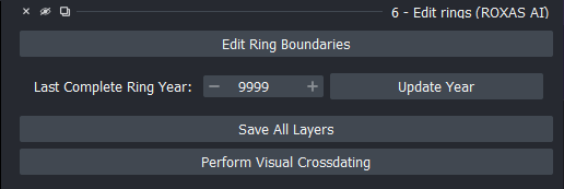
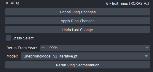
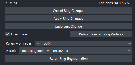
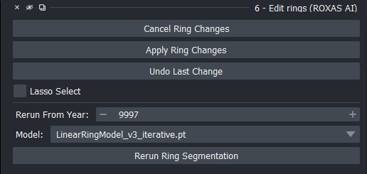
Figure 8: Rings layer editor widget in its four operational states: (A) Startup, (B) Vector polyline boundary editing, (C) Lasso vertex selection and deletion, and (D) Targeted model re-segmentation workflow.

How It Works

1. Mutual Editing Exclusion & Layer Guards: Enters vector polyline editing mode (Rings Modification) while automatically hiding cell layers (.cells) and CWT visualization circles ([<sample>] CWT Circles) to prevent layer conflicts. Exiting ring editing mode automatically restores cell and CWT layer visibilities.
2. Converts the raster ring mask into continuous polyline shapes representing each ring boundary, enforcing strict left-to-right vertex ordering (rearrange_coordinates) and proximity-based vertex insertion to avoid self-intersecting loops.
3. Displays real-time calendar year labels (Rings Years overlay) along the sample.
4. Allows interactive vertex adjustments, insertion of missing boundaries, or deletion of false boundaries using napari shape tools.
5. Fine-Positioning & Bulk Movement:
   • Fine Nudging (1 px): Press Ctrl + Arrow keys to nudge all selected boundary vertices by 1 pixel.
   • Fast Nudging (10 px): Press Ctrl + Shift + Arrow keys to nudge all selected boundary vertices by 10 pixels.
   • Bulk Movement: Multiple boundaries can be selected simultaneously and moved manually or with nudging operations with full transform undo tracking.
   • Transformations: The entire rings layer can be selected and moved manually or with nudging operations.
6. Lasso Selection Priority on Overlapping Rings:
   • When boundaries overlap or share coordinates, deleting vertices with the lasso tool selectively removes vertices strictly from the topmost ring boundary (highest shape index), leaving underlying boundaries intact.
7. Adding Missing & Wedging/Incomplete Rings:
   • Missing Rings: Select a ring boundary with the feature selection tool and copy-paste it; the added ring boundary will be perfectly on top.
   • Wedging / Incomplete Rings:
     1. Copy-paste the ring boundary that shares the common portion of the ring contour.
     2. Use the lasso tool to delete the diverging/erroneous vertices from the top ring.
     3. Extend the top ring by manually tracing the actual wedging trajectory.
8. Undo Mechanism:
   • Full 50-step undo history (Ctrl+Z or Undo Last Change button) restoring boundary geometries, calendar year metadata, deleted vertex markers, and affine transform states.
9. Annotated Image Generation:
   • Configurable annotated overview scans (<sample>_annotated.jpg) overlaid with ring boundaries, year labels, and optional semi-transparent cell lumen overlays (cell_opacity, cell_fill_color, year_label_size, scale factor, JPEG quality).
10. Rerun Ring Segmentation:
    • Re-runs the ring boundary detection AI specifically below a corrected reference ring boundary.
11. Customizable Tolerances & Colors:
    • Polyline smoothing tolerances, line thickness, and boundary colors can be customized in ZZ - Settings (see Technical Reference: Visualization Settings).

Files and Layers Saved

• In-Memory Modifications: Adding, deleting, or nudging ring boundaries updates the <sample>.rings labels layer and Rings Years text overlay upon clicking Apply Ring Changes, marking the .rings layer as modified.
• Annotated Overview Image (<sample>_annotated.jpg): Automatically re-drawn and saved directly to disk whenever Update Year is clicked, reflecting the new ring year labels and boundary positions.
• Ring Table Synchronization (<sample>.rings_table.csv): When ring changes or year updates are applied, existing ring tables are updated to keep ring numbers and years consistent.
• Saving to Disk: Clicking Save All Layers (or using 8 - Save Cells & Rings Editing) writes the updated <sample>.rings.tif mask and <sample>.metadata.json (outermost year rings_outmost_complete_year, ring count rings_count) to disk. Manual saves do not redraw <sample>_annotated.jpg to keep saving instantaneous.

Key Controls & Options

• Last Complete Ring Year (SpinBox): Specifies the calendar year of the outermost complete annual ring. Supports calendar years from -100,000 (prehistoric/BCE dates) up to 9,999 (CE).
• Update Year: Updates the calendar year metadata, recalculates ring year labels in the viewer, and redraws the annotated overview image (<sample>_annotated.jpg) with the new ring years.
• Edit Ring Boundaries: Enters vector polyline editing mode and displays boundary lines.
• Lasso Select: Checkbox activating lasso-based vertex selection.
• Delete Selected Ring Vertices: Removes all boundary vertices enclosed by the lasso selection (deleting from the topmost boundary when layers overlap).
• Undo Last Change: Reverts the most recent shape edit, deletion, or movement (also available via Ctrl+Z).
• Perform Visual Crossdating: Opens the Visual Cross-Dating widget directly for the active sample (see 7 - Visual Cross-Dating).
• Rerun Model from Year Workflow: Re-evaluates and automatically re-detects ring boundaries starting below a corrected reference ring boundary:
  1. Initial Detection: Run standard automated tree-ring segmentation on the sample (via 3A - Detect Cells & Rings).
  2. Inspect Boundaries: Starting from the top (bark side), inspect the detected ring boundaries.
  3. Correct Boundary Error: If you notice a series of systematically incorrectly defined ring boundaries (e.g., jumps, jags; frequently starting from the top ring), delete the first/top erroneous boundary and manually redraw it correctly using the shape editing tools; then click Apply Ring Changes.
  4. Re-enter Editing & Set Year: Click Edit Ring Boundaries again and set Rerun From Year: to the calendar year of the manually added or corrected ring boundary.
  5. Select Model & Re-run: In the Model: dropdown, choose the ring model checkpoint (e.g., LinearRingModel_v3_iterative.pt) and click Rerun Ring Segmentation.
  6. Iterative Re-detection: All ring boundaries below the manually corrected ring boundary are automatically re-detected and reconstructed based on the corrected boundary geometry.
• Apply Ring Changes: Validates topology, updates .rings labels, updates .rings_table.csv, and saves year metadata.
• Cancel Ring Changes: Reverts to original ring boundaries and restores previous layer states.
• Save All Layers: Persists all modified sample layers, metadata, and the annotated overview image directly to disk (see 8 - Save Cells & Rings Editing).

Dedicated Shortcuts

For a complete summary of all shortcuts across the application, see the Shortcuts Reference.

Action	Dedicated Shortcut	Scope
Fine Nudge Boundary (1 px)	Ctrl + ↑ / ↓ / ← / →	Active in 6 - Edit rings (Selected Boundaries)
Fast Nudge Boundary (10 px)	Ctrl + Shift + ↑ / ↓ / ← / →	Active in 6 - Edit rings (Selected Boundaries)
Delete Lasso Vertices	Delete or Backspace	Active in 6 - Edit rings (Lasso Mode)
Undo Last Change	Ctrl + Z	Active in 6 - Edit rings

---

7 - Visual Cross-Dating

The Cross-Dating Plotter Widget couples tree-ring width (TRW) time series derived from detected rings with master reference chronologies in an interactive plotting environment.

A: Standard ViewB: Candidate Alignment OptionsC: Rendered Reference Plot

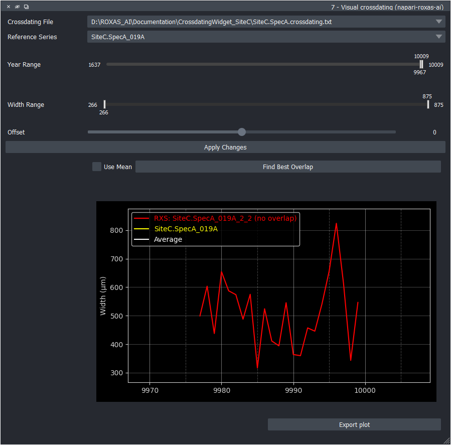
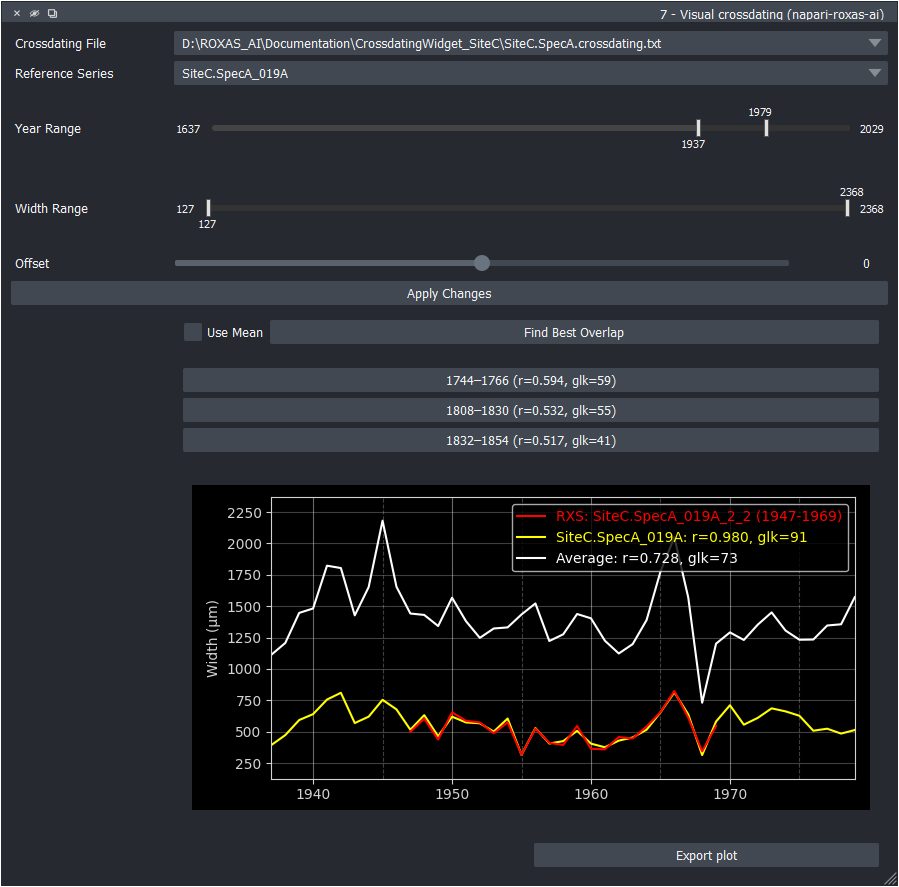
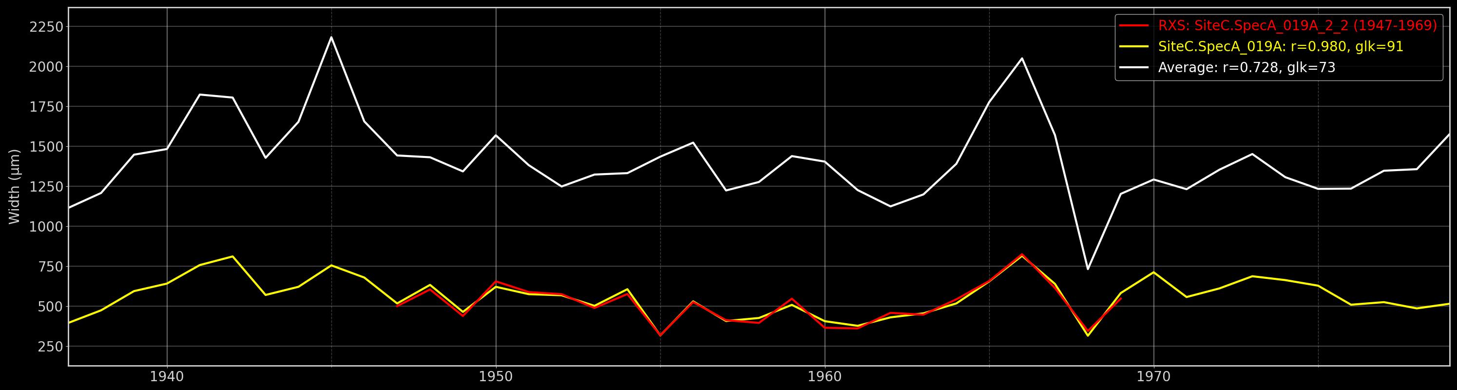
Figure 9: Visual cross-dating plotter synchronizing sample ring-width series with reference chronology: (A) Standard floating plotter interface with ±10-year buffer, (B) Candidate alignment suggestions ranked by correlation (r) and Gleichläufigkeit (GLK), and (C) Rendered reference series plot exported as <sample>_ReferenceSeries.jpg.

How It Works

• Computes mean ring width (MRW) from the ring boundaries currently in the viewer.
• Renders dual interactive curves in a Matplotlib canvas: the sample series and the reference series.
• Supports calendar year ranges spanning from prehistoric/BCE periods down to -100,000 up to 9,999 (CE).
• Formats negative/prehistoric years as plain integers on axes and dynamically calculates gridline steps (e.g., 10, 20, 50, 100, 200, 500, 1000 years) based on the active viewing span.
• Floating Presentation & Sizing Grip: Opens automatically as a floating window centered on the active screen with a 100 px margin and a prominent diagonal sizing grip, allowing flexible side-by-side positioning with the napari viewer.
• Year Range & Offset Slider Interaction:
  • The standard view automatically centers on the target ROXAS sample series with a default buffer of \(\pm 10\) years on each side.
  • To slide the sample series beyond this initial \(\pm 10\) year window, adjust the Year Range slider to expand the visible time span. Expanding the Year Range slider automatically widens the allowable range of the Offset slider, allowing you to slide the series across decades or centuries.
  • Both the Year Range (X-axis) and Width Range (Y-axis) sliders use split handle labels (lower bound below the bar, upper bound above) to prevent label overlap when handles are close together.
• Auto-Offset Alignment & Candidate Selection:
  • The Find Best Overlap feature scans offsets across the active time window to automatically maximize correlation (\(r\)) and sign agreement (GLK).
  • Use Mean Checkbox: When checked, aligns the sample against the overall mean of all reference series in the file rather than a single individual column.
  • Interactive Candidate Alignment Buttons: In addition to applying the top-ranked alignment, ROXAS AI generates interactive buttons for alternative candidate alignments with their year spans and statistical scores (e.g., 1900–1980 (r=0.642, glk=72)). Clicking any candidate button instantly shifts the plot to that dating and updates the button to allow swapping back.
• Uniform Scaling Across Reference Plots:
  • Reference plot figures are generated with a standardized vertical height of 800 pixels and a constant horizontal scale of 70 pixels per year of overlap (min(50 + (20 + overlap_years) * 70, 65000)). This guarantees identical visual scale across different samples and chronologies.
• Reference Plot Creation:
  • Reference plot images (<sample>_ReferenceSeries.jpg) are generated and saved when clicking Export Plot, clicking Apply Changes, or automatically during batch measurement runs in 9B - Batch Measure & Update.
• Statistical Synchrony Metrics:
  • Computes Correlation coefficient (\(r\)), Gleichläufigkeit (GLK / % sign agreement), and \(t\)-value / statistical significance in real time.

Cross-Dating Files Discovery & Folder Hierarchy Traversal

When a sample's tree-ring layer is selected in napari, the widget automatically locates associated cross-dating text files using an upward directory traversal algorithm:

1. Starting Point: The search begins in the directory containing the active sample scan (determined from sample_stem_path, the layer's file path, or the global project_directory).
2. Search Direction (Strictly Upward):
   • The search is strictly upward (from the sample's directory towards the root of the file system).
   • The widget does not search downwards into subdirectories.
3. Search Pattern & Prefix Requirements:
   • The search matches files using the pattern *<crossdating_file_extension>, where <crossdating_file_extension> is the configured extension in settings.json under file_extensions.crossdating_file_extension (by default [".crossdating", ".txt"], which concatenates to .crossdating.txt).
   • Prefixes are supported: Because of the leading wildcard *, any custom prefix before the extension is detected (e.g., rings_series.crossdating.txt, siteA_chronology.crossdating.txt, or conifer_ref.crossdating.txt).
   • Suffixes are NOT supported after the extension: The file must strictly end with the configured cross-dating extension (e.g., .crossdating.txt). If a file has an additional suffix after the extension (e.g., .crossdating.txt.bak) or a different extension (such as .csv when .crossdating.txt is configured), it will not be matched unless the extension setting in settings.json is updated.
4. Upward Directory Tree Traversal Process:
   • The widget first inspects the sample's immediate folder (current_path.glob(pattern)).
   • If one or more matching cross-dating files are found in that folder, search stops and those files are loaded.
   • If no matching file is found, it moves up to the parent directory (current_path = current_path.parent) and repeats the check.
   • The upward search continues through parent folders until matching files are found or it reaches the file system root.
   • Architectural Workflow: This allows placing a single global reference file at the project root directory (e.g., <project_root>/rings_series.crossdating.txt) to serve all samples in subfolders, or placing local reference files in specific sample subfolders (e.g., <project_root>/SiteA/rings_series.crossdating.txt), which automatically take priority for samples located within SiteA.

Behavior When Multiple Cross-Dating Files Are Present

• Multiple Files in the Same Directory:
  • If two or more matching cross-dating files exist within the first directory where matches are found (e.g., <project_root>/rings_series_site1.crossdating.txt and <project_root>/rings_series_site2.crossdating.txt):
    • All discovered cross-dating files are collected and populated into the Crossdating File dropdown combobox (_crossdating_file_combo).
    • The widget automatically selects the first file in the list by default.
    • Users can freely switch between files using the Crossdating File dropdown. Selecting a different file immediately re-reads the dataset, recalculates the series average, updates the Reference Series dropdown with all series columns from that file, and refreshes the plot.
• Files in Different Directory Levels:
  • Because traversal stops at the first directory containing matches, a cross-dating file located in a sample's local subfolder takes precedence over a cross-dating file located in parent or root directories.

Files and Layers Saved

• In-Memory Modifications: Clicking Apply Changes updates the year labels on the Rings Years text overlay, shifts .rings label indices, and marks the .rings layer as modified with the new outermost year.
• Annotated Overview Image (<sample>_annotated.jpg): Automatically re-generated and saved to disk with updated ring calendar year labels upon clicking Apply Changes.
• Reference Series Plot (<sample>_ReferenceSeries.jpg): Generated and saved to disk when clicking Apply Changes or Export Plot (or automatically during batch measurement updates via 9B - Batch Measure & Update), plotting sample mean ring width (MRW) against the selected reference chronology.
• Metadata (<sample>.metadata.json): Updated with the validated outermost year (rings_outmost_complete_year) and the selected reference series column (reference_series). The cross-dating file path itself is not stored, enabling portable directory hierarchies.
• Ring Table Synchronization (<sample>.rings_table.csv): If measurement tables already exist on disk, their YEAR column is automatically updated to reflect the new dating.

Key Controls & Options

• Crossdating File Dropdown: Selects among multiple detected cross-dating files in the directory tree.
• Reference Series Dropdown: Selects from individual series, site chronologies, or the auto-computed "average" column from the active cross-dating file. Automatically prioritizes columns whose names match the active sample stem.
• Use Mean Checkbox: Toggles whether auto-alignment computes the best overlap against the composite average of all columns in the cross-dating file instead of the selected reference series column.
• Find Best Overlap Button: Automatically scans temporal shifts to align sample and reference curves by maximizing correlation and sign agreement (GLK), generating candidate alignment buttons.
• Candidate Alignment Buttons: Interactive buttons created below the alignment row displaying the top alternative alignment year spans and scores (e.g., 1900–1980 (r=0.642, glk=72)). Clicking any button shifts the plot to that dating and swaps previous alignment data for easy toggling.
• Year Range & Width Range Dual Sliders: Interactively set X (calendar year range, supporting -100,000 to 9,999) and Y (ring width in \(\mu\text{m}\)) viewing windows, using split handle labels to avoid label overlap.
• Offset Slider: Manually shifts sample dating relative to the reference chronology. Expanding the Year Range slider broadens the available offset adjustment window.
• Apply Changes Button: Confirms the adjusted temporal offset, updates ring boundary year numbering, shifts the .rings layer labels, records the new outermost year in sample metadata (rings_outmost_complete_year), synchronizes .rings_table.csv, regenerates <sample>_annotated.jpg, and exports <sample>_ReferenceSeries.jpg.
• Export Plot Button: Saves the current cross-dating plot as a publication-ready <sample>_ReferenceSeries.jpg image in the sample directory and records the validated reference series in <sample>.metadata.json.

---

8 - Save Cells & Rings Editing

The Samples Saving Widget writes modified cell masks, ring boundaries, and updated sample metadata from napari back to their respective files on disk.

Figure 10: Samples saving widget interface.

How It Works

• Gathers data, layer parameters, and metadata from active napari layers.
• Formats and writes .cells.png (8-bit or 16-bit label rasters) and .rings.tif to disk.
• Unsaved Changes Tracking: Layers loaded from disk start out unmodified. Manual edits (vector/raster cell modifications, adding/moving/deleting rings, changing outermost ring year, applying cross-dating offsets) and freshly run AI segmentations mark the corresponding layers as modified (layer.metadata["is_modified"] = True).
• Targeted Saving: Save All Layers checks which layers have unsaved edits and saves only those modified layers to disk, skipping unmodified files.
• Explicit Save Status Notifications: Reports exactly what was written:
  • "Saved cells layer." (when only .cells was modified)
  • "Saved rings layer." (when only .rings was modified)
  • "Saved cells and rings layers." (when both were modified)
  • "No unsaved changes in cells or rings layers." (when no changes were pending)
• Fast Saving Decoupled from Overview Rendering: Manual layer saving does not redraw the annotated overview image (<sample>_annotated.jpg), ensuring saves complete in milliseconds without disk or CPU overhead. The annotated overview image is automatically regenerated at key workflow checkpoints instead: AI segmentation (3A/3B), Update Year (6), Apply Changes in cross-dating (7), and trait measurement (9A/9B).
• Updates <sample>.metadata.json with updated ring counts, outermost year, and timestamps.
• Operates in a non-blocking background worker thread.

Files and Layers Saved

• Cell Masks (<sample>.cells.png): Written to disk if .cells has unsaved changes.
• Ring Masks (<sample>.rings.tif): Written to disk if .rings has unsaved changes.
• Metadata (<sample>.metadata.json): Synchronized with layer metadata parameters (outermost ring year rings_outmost_complete_year, ring count rings_count, layer timestamps).
• Overview Image Note: <sample>_annotated.jpg is not overwritten on manual save, keeping layer saving instantaneous.

Key Controls

• Save Selected Layers: Saves only the layers currently highlighted in the napari layer list.
• Save All Layers: Saves only the .cells and .rings layers with unsaved changes and reports what was written ("Saved cells layer.", "Saved rings layer.", or "Saved cells and rings layers."). Without changes, nothing is written and "No unsaved changes in cells or rings layers." is shown.
• Progress Bar: Shows disk write progress, scaled to the number of layers actually saved.

---

9A - Measure Cells & Rings (Individual Image)

The Single Sample Measurements Widget computes the full suite of Quantitative Wood Anatomy (QWA) metrics for the sample currently loaded in napari.

A: Measurement ControlsB: In-Viewer CWT QA Layer

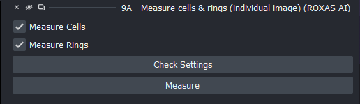
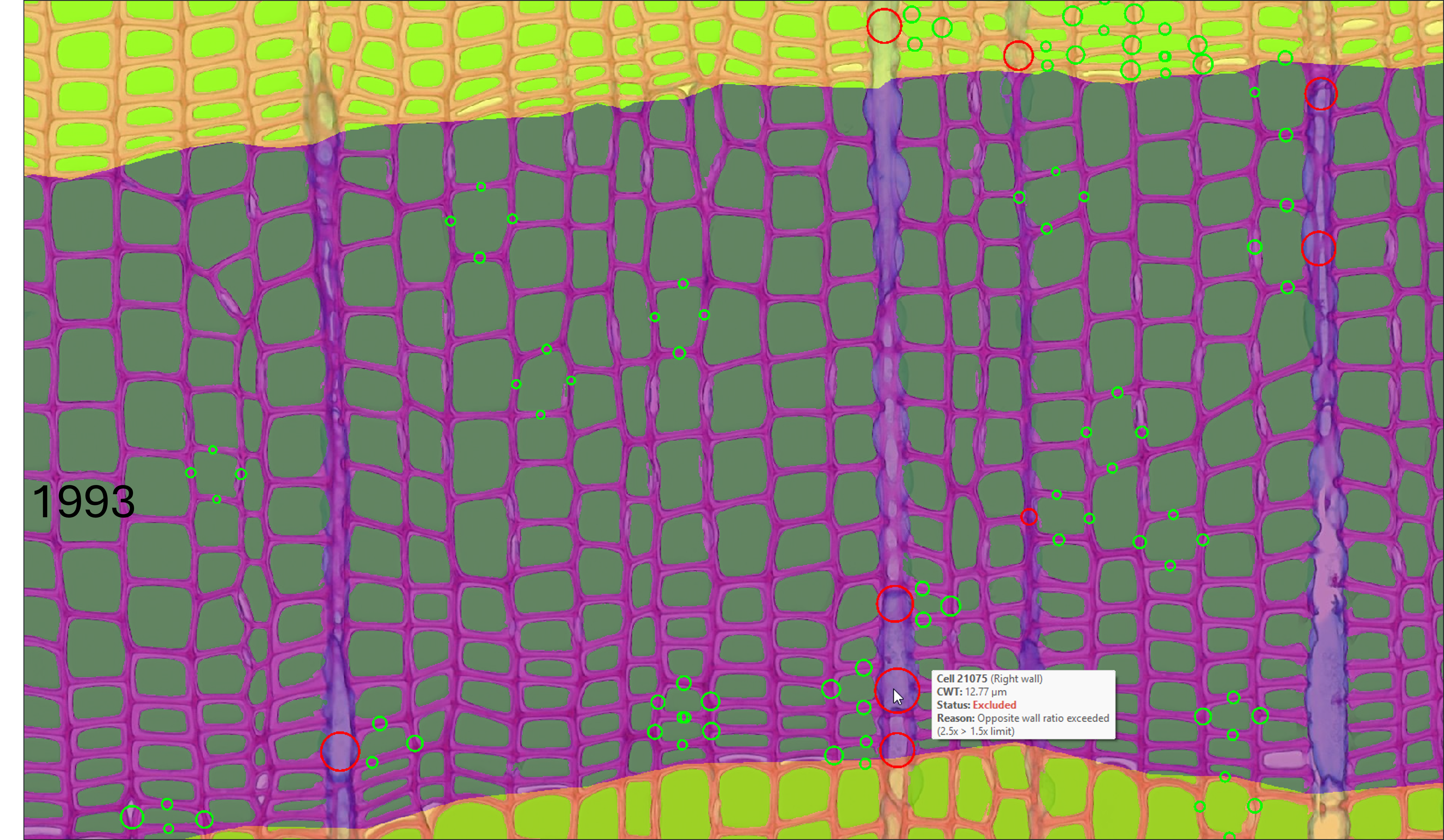
Figure 11: Single sample measurements and quality assurance interface: (A) Trait measurement controls and (B) Interactive CWT Quality Assurance shapes overlay in the napari viewer displaying color-coded inclusion (green)/exclusion (red) circles and hover tooltips.

How It Works

• Combines the .cells lumen mask, .rings boundary geometry, and spatial resolution metadata (\(\mu\text{m}/\text{px}\)) to compute anatomical and ring-width traits:
  • Cell-Level Metrics: Lumen dimensions, conduit hydraulic diameter, theoretical conductance, and cell wall thickness. See Cell-Level Output (.cells_table.csv) for complete variable definitions.
  • Ring-Level Aggregates: Mean ring width, cell count, cell density, conductive area percentage, Mork's index, and anatomical density. See Ring-Level Output (.rings_table.csv) for complete variable definitions.
  • CWT Quality Control & QA Layer: Applies multi-stage outlier and ray-artifact filtering (see CWT Quality Control & Filtering) and generates a non-destructive [<sample>] CWT Circles Shapes layer with color-coded circles and interactive hover tooltips (displaying Cell ID, sector, thickness, status, and filter reasons) for visual quality control.
• Outputs semicolon-delimited CSV tables (<sample>.cells_table.csv, <sample>.rings_table.csv) and the CWT quality assurance dataset (<sample>.cwt.json).
• Always Re-creates Annotated Image: Re-creates and saves an updated annotated overview image (<sample>_annotated.jpg) overlaid with ring boundaries and years whenever measurements are performed, ensuring the annotated image remains strictly in line with the measurements.

Files and Layers Saved

• Cell Measurement Table (<sample>.cells_table.csv): Saved directly to disk with comprehensive lumen and cell wall thickness metrics per detected cell instance (when Measure Cells is enabled).
• Ring Measurement Table (<sample>.rings_table.csv): Saved directly to disk with ring-width and ring-level aggregate anatomical traits per calendar year (when Measure Rings is enabled).
• CWT Visualization Data (<sample>.cwt.json): Saved directly to disk with circle coordinates, thickness values, filter statuses, and exclusion reasons.
• CWT Circles Shapes Layer ([<sample>] CWT Circles): Added to the napari viewer for interactive visual quality control.
• Annotated Overview Image (<sample>_annotated.jpg): Automatically re-generated and saved to disk with synchronized ring boundaries, calendar years, and cell lumen overlays.
• Layer Feature Tables: In-memory feature tables on .cells and .rings layers are updated, allowing interactive inspection of properties directly within napari.

Key Controls

• Measure Cells / Measure Rings: Checkboxes selecting whether to measure cell anatomical metrics, tree-ring boundary metrics, or both.
• Check Settings Button: Launches the Settings window (see ZZ - Settings) as a floating widget that appears maximized with a comfortable margin on top of napari, automatically expanding and scrolling to the measurement parameters.
• Measure Button: Launches analysis in a background worker with an animated processing spinner (Processing | / - \), writes measurement tables, .cwt.json, and the updated annotated image, cleans non-measured edge artefacts from the cell mask, attaches measurements to layer properties for interactive table inspection, and marks layers as saved (_is_dirty = False).

---

9B - Batch Measure & Update

The Batch Sample Measurements Widget runs high-throughput anatomical trait extraction, annotated image generation, and reference plot synchronization across all samples in a project folder.

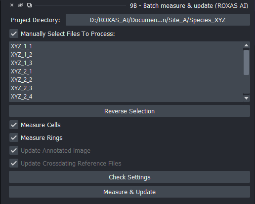
Figure 12: Batch sample measurements and update interface.

How It Works

• Discovers all matched pairs of .cells and .rings files in the project directory.
• Real-Time Dynamic Sync: Listens to project directory and project file changes so that samples generated by earlier steps (such as preparation or batch segmentation) appear immediately in the file list without closing or reopening the widget.
• Reads image scale and configuration from each sample's .metadata.json.
• Computes cell-level and ring-level measurement tables in batch mode.
• Writes <sample>.cells_table.csv, <sample>.rings_table.csv, and <sample>.cwt.json directly to each sample folder.
• Generates or updates annotated overview scans (<sample>_annotated.jpg) and cross-dating reference plots (<sample>_ReferenceSeries.jpg).
• How Reference Plot Updates Work: When generating <sample>_ReferenceSeries.jpg, ROXAS AI extracts the sample's measured mean ring width (MRW) series from <sample>.rings_table.csv (or calculates it from the .rings mask). It discovers available cross-dating files in the directory hierarchy by searching strictly upwards from the sample folder for files matching the configured cross-dating file extension (e.g., *.crossdating.txt). To determine which reference series to plot against:
  • If a specific reference series was previously saved in <sample>.metadata.json (reference_series), and that column exists in one of the discovered cross-dating files, it uses that stored reference series.
  • If no reference series is stored (or reference_series is "NA" or no longer present in the files), ROXAS AI automatically searches the series columns of the discovered cross-dating files for the best name match with the sample name.
  • If a matching reference series is identified, the plot is rendered and <sample>.metadata.json is updated with the selected reference_series. If no cross-dating files or matching series are found, reference plot creation is safely skipped.

Files and Layers Saved

• Cell Measurement Tables (<sample>.cells_table.csv): Saved to disk for each processed sample when Measure Cells is enabled.
• Ring Measurement Tables (<sample>.rings_table.csv): Saved to disk for each processed sample when Measure Rings is enabled.
• CWT Visualization Files (<sample>.cwt.json): Saved to disk for each processed sample when cell measurements are run.
• Annotated Overview Images (<sample>_annotated.jpg): Saved or updated on disk for each sample when Update Annotated image is active (or locked on during measurements).
• Reference Series Plots (<sample>_ReferenceSeries.jpg): Saved or updated on disk for each sample when Update Crossdating Reference Files is active (or locked on during measurements), plotting sample MRW curves against their validated reference chronologies.
• Metadata (<sample>.metadata.json): Synchronized with updated analysis timestamps and measurement parameters.

Linked Operations Logic (File Synchronization)

To prevent dataset inconsistencies, ROXAS AI enforces linked operation synchronization:

• When Measure Cells or Measure Rings is checked, the update checkboxes for Update Annotated image and Update Crossdating Reference Files are automatically locked ON (checked and disabled).
• Reason: Any recalculation of anatomical traits or ring boundaries changes the underlying metrics and years; locking the image and plot updates guarantees that measurement tables, annotated scan images, and crossdating plots remain 100% synchronized with the new measurements.
• When both measurement options are unchecked, the update checkboxes are unlocked, enabling standalone batch generation/updating of annotated images and reference plots across the project directory without re-running full measurements.

Key Controls

• Project Directory Button: Displays and allows switching the active project directory (triggering the same global project directory selection dialog).
• File Selection Mode: Toggle between processing all samples and handpicking subsets (Select individual files:).
• Reverse Selection: Inverts current sample selections in the list.
• Operation Checkboxes:
  • Measure Cells: Extracts cell lumen and cell wall thickness metrics to <sample>.cells_table.csv and saves <sample>.cwt.json.
  • Measure Rings: Extracts ring-width and ring-level aggregate metrics to <sample>.rings_table.csv.
  • Update Annotated image: Generates/updates <sample>_annotated.jpg with ring boundaries, year labels, and cell overlays.
  • Update Crossdating Reference Files: Generates/updates standardized <sample>_ReferenceSeries.jpg plots.
• Check Settings Button: Opens the floating Settings window focused directly on the measurement parameters.
• Measure & Update Button: Runs batch extraction and updates with real-time progress bar tracking.

---

ZZ - Settings

The Settings Widget is a visual preferences manager that allows adjusting global defaults, file extensions, visualization parameters, and hardware settings without manual editing of JSON files.

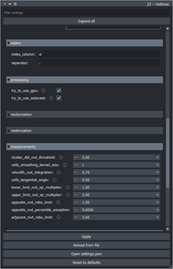
Figure 13: Global settings manager widget with collapsible categories.

How It Works

• Directly manages settings.json with dedicated input editors matching each data type (spinboxes, color selectors, list editors, checkboxes).
• Prevents syntax errors, invalid datatypes, or formatting corruption.
• Floating Presentation & Sizing Grip: Opens automatically as a floating window centered on the active screen with comfortable 50 px vertical margins and a prominent diagonal sizing grip.
• Live Search & Filter: Instant multi-term search filtering finds matching setting entries across all categories (e.g., typing "gpu" finds try_to_use_gpu, "cwt" finds cwt_visualization options), displaying the count of matching items and offering a clear button.
• Expand All / Collapse All: Toggles the expansion state of all setting categories at once.
• Immediate Application Without Restart: Applying changes writes settings.json to disk and immediately notifies all active widgets and listeners in the running session.

Key Settings Categories

1. File Extensions:
   • Standardized file suffixes for scans, cell masks, ring masks, metadata files, CWT files (.cwt.json), cross-dating chronologies, and tables.
2. Hardware & Processing:
   • try_to_use_gpu: Toggle CUDA / MPS / XPU acceleration for deep-learning segmentation.
   • Worker thread and batch settings.
3. Visualization & Vectorization:
   • Default colormaps for cell lumen layers.
   • Ring color sequence (alternating colormap for adjacent annual rings).
   • Display line widths and point sizes.
   • Annotated image parameters (cell_opacity, cell_fill_color, year_label_size).
4. CWT Quality Assurance & Visualization:
   • enabled: Toggle creation and display of the CWT circles layer.
   • sample_interval: Stride interval for cell sampling (default: 25).
   • included_color / excluded_color: Custom display colors for included and excluded measurement circles.
   • edge_width: Line width of visualization circles.
5. Measurement Defaults:
   • Default CWT integration widths, smoothing kernel sizes, IQR outlier rejection multipliers, opposite-wall percentile exception (opposite_cwt_percentile_exception, default 0.60), and cluster thresholds.
6. Metadata Schema:
   • Default metadata prompts and fields presented during sample preparation.

Key Controls

• Search Bar: Live filter box matching any part of setting names or paths across categories.
• Expand all / Collapse all: Expands or collapses all category groups.
• Apply: Persists all settings to disk and applies them immediately across the running session.
• Reload from file: Discards unapplied UI changes and reloads current settings from settings.json.
• Open settings.json: Opens the raw configuration file in the system default text editor.
• Reset to defaults: Resets all settings to the factory default configuration (with confirmation prompt).

Troubleshooting: Settings Not Updating After an App Upgrade

When updating napari-roxas-ai over an older installation, existing configurations in settings.json are automatically preserved so custom user settings are not lost.

• Reset from the UI: To load the newest defaults, open the ZZ - Settings widget and click Reset to defaults.
• Clean Reinstall: For step-by-step instructions on performing a complete clean reinstall, see the Installation Guide.