Tutorials & Workflows¶

Step-by-step guides for quantitative wood anatomy (QWA) and dendrochronological analysis using ROXAS AI in napari.

Choosing the Right Workflow

Interactive / Single-Sample Workflow (Section 1 & 2): Best for detailed visual inspection, manual touch-ups of cell lumens and tree-ring boundaries, and interactive visual cross-dating using the Manual Editing Group (Ctrl+Shift+M).
Batch Processing Workflow (Section 3): Best for multi-sample datasets where segmentation, measurements, quality assurance data (.cwt.json), and overview plots are run automatically in sequence using the Batch Operations Group (Ctrl+Shift+B).

1. Quickstart: 5-Minute Single Sample Walkthrough¶

This fast-track walkthrough guides you from raw anatomical image to measured cellular and tree-ring traits using the bundled conifer sample and the Manual Editing Group (Ctrl+Shift+M).

flowchart TD
    S1["Step 1: Launch napari-roxas & Open Sample Data"] --> S2["Step 2: Run Deep Learning Detection (Widget 3A)"]
    S2 --> S3["Step 3: Quick Visual Verification & Curation (Widgets 5 & 6)"]
    S3 --> S4["Step 4: Extract Cell & Ring Measurements (Widget 9A)"]

Step 1: Launch ROXAS AI & Open Built-in Sample Data¶

Open your terminal or conda prompt with the roxas-ai environment active and start the application:
```
napari-roxas
```
This starts napari, registers viewport navigation shortcuts (WASD, Q/E), and docks the Manual Editing Group in the right sidebar.
Navigate to the top menu: File > Open Sample > ROXAS AI.
ROXAS AI loads the conifer cross-section scan along with pre-configured spatial metadata (\(\text{px}/\mu\text{m}\)).

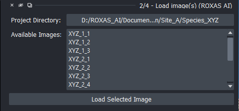
Figure 1: Conifer sample dataset loaded into the napari viewer.

Step 2: Run Deep Learning Detection¶

In the docked sidebar, locate 3A - Detect cells & rings (individual image).
Select the deep-learning models:
- Cells Model: linear_cells_model (ResNet-50 U-Net architecture)
- Rings Model: LinearRingModel_v3_iterative.pt (Iterative boundary regression)
Click Run Segmentation.

!!! info "Automatic Model Weights Download" If you are running segmentation for the first time, ROXAS AI automatically downloads pre-trained model weights in the background and caches them locally for all subsequent runs.

Deep-learning inference populates the interactive napari layers:
- <sample>.cells: Labeled cell lumen instances (Labels layer).
- <sample>.rings: Labeled annual tree-ring bands and boundaries (Labels layer).
- Rings Years: Persistent calendar year text overlay along detected boundaries (Points layer).

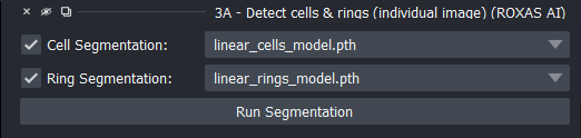
Figure 2: Automated cell lumen and tree-ring boundary segmentation layers.

Step 3: Quick Visual Verification & Curation¶

Navigate across the sample using single-key shortcuts:
- Pan: W, A, S, D or Arrow keys (hold Shift for fast panning at 400 px/step).
- Zoom: Q to zoom out, E to zoom in (\(0.25\times\) zoom step).
Expand 5 - Edit cells or 6 - Edit rings in the sidebar to make quick adjustments:
- Cell Editing (Raster Mode): Hold Ctrl + Mouse Wheel to dynamically resize the brush (1–100 px); hold Ctrl + Double-Click to toggle between brush and eraser. Press Ctrl+Z to undo any stroke.
- Ring Editing: Select a boundary and press Ctrl + Arrow keys to nudge it by 1 pixel (or Ctrl + Shift + Arrow keys for 10 pixels). Press Ctrl+Z to undo.

Step 4: Extract Cell & Ring Measurements¶

In the sidebar, scroll to 9A - Measure cells & rings (individual image).
Verify that Measure Cells and Measure Rings are checked.
(Optional) Click Check Settings to review or customize measurement parameters and quality control thresholds.
Click Measure.
The measurement engine outputs comprehensive semicolon-delimited CSV tables, CWT quality assurance data, and an updated overview image in the project directory:
- <sample>.cells_table.csv: Lumen Area (LA), Cell Wall Thickness (CWTALL, CWTRAD, CWTTAN), Mork's Index (RTSR), Theoretical Hydraulic Conductance (KH), and Hydraulic Diameter (DH).
- <sample>.rings_table.csv: Mean Ring Width (MRW), Cell Count (CNO), Mean Lumen Area (MLA), Cell Density (CD), and Relative Anatomical Density (RWD).
- <sample>.cwt.json: Circle geometries, wall thickness values, inclusion/exclusion status, and filter reasons for sampled cells.
- [<sample>] CWT Circles Shapes Layer: Non-destructive viewer layer displaying green (included) and red (excluded) measurement circles. Hover over any circle to view an interactive tooltip with Cell ID, wall sector, thickness (\(\mu\text{m}\)), status, and exclusion reason.
- <sample>_annotated.jpg: High-resolution scan automatically regenerated with overlaid ring boundaries, calendar year labels, and cell lumen highlights.
- Layer Feature Tables: In-memory feature tables on .cells and .rings layers are updated, allowing interactive trait inspection directly inside napari.

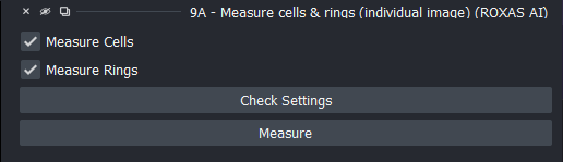
Figure 3: Single sample measurement interface and extracted output tables.

2. Standard Workflow: Tree-Ring & Cell Anatomy Time Series¶

This comprehensive protocol describes the standard end-to-end workflow for generating publication-quality dendroclimatic and wood anatomical time series from raw microsections or surface scans.

flowchart TD
    P1["Step 1: Project Setup & Image Preparation (Widget 1 / Ctrl+Shift+B)"] --> P2["Step 2: Loading & Automated Segmentation (Widgets 2/4 & 3A / Ctrl+Shift+M)"]
    P2 --> P3["Step 3: High-Accuracy Lumen & Cell Wall Editing (Widget 5)"]
    P3 --> P4["Step 4: Tree-Ring Editing & Boundary Curation (Widget 6)"]
    P4 --> P5["Step 5: Visual Cross-Dating (Widget 7)"]
    P5 --> P6["Step 6: Save Annotations & Metadata (Widget 8 / Save All Layers)"]
    P6 --> P7["Step 7: Trait Extraction & Chronology Export (Widget 9A)"]

Step 1: Project Setup & Image Preparation¶

Launch napari via napari-roxas.
Press Ctrl + Shift + B to open the Batch Operations Group.
In 1 - Prepare project images for analysis:
- Select your project directory (or use 0 - Define project directory).
- Enter physical spatial resolution (\(\text{px}/\mu\text{m}\) or \(\mu\text{m}/\text{px}\)), anatomy type (conifer), geometry (linear), and the outermost complete calendar year.
- (Optional) Click Start Processing Crossdating Files to import reference ring-width chronologies (.rwl, .tuc, or tabular .txt/.csv). Series names of up to 8 characters are parsed automatically.
Click Prepare Images. The images are standardized to <sample>.scan.<ext>, initialized with <sample>.metadata.json, and parsed reference chronologies saved to rings_series.crossdating.txt.

Step 2: Loading & Automated Segmentation¶

Press Ctrl + Shift + M to switch to the Manual Editing Group.
In 2/4 - Load image(s), select your prepared sample from the dropdown (or double-click to load). Single-image enforcement ensures clean memory management.
In 3A - Detect cells & rings (individual image), select the neural network models and click Run Segmentation.
Cell lumen masks (<sample>.cells), ring boundary contours (<sample>.rings), and the Rings Years calendar year text overlay will populate as interactive napari layers in the viewer.

Figure 4: Automated cell and ring predictions visualized in napari.

Step 3: High-Accuracy Lumen & Cell Wall Editing¶

Refine cell lumen annotations using 5 - Edit cells in the Manual Editing group.

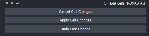
Figure 5: Cell layer editor displaying raster brush/eraser controls and vector polygon conversion.

Raster vs. Vector Editing Modes¶

Mode	Best Used For	Tooling & Mechanics	Dedicated Shortcuts
Raster Mode	Rapid mask cleaning, separating merged cells, filling voids	Pixel brush, eraser, and paint bucket operating directly on the integer label raster.	`Ctrl` + Wheel (Brush size: 1–100 px) `Ctrl` + Double-Click (Switch brush/eraser) `Ctrl`+`Z` (Undo stroke)
Vector Mode	High-precision boundary adjustments, polygon vertex editing, batch lasso deletion	Interactive polygon contours with vertex dragging, shape addition, and Lasso Delete.	`Delete` / `Backspace` (Delete lasso selection) `Ctrl`+`Z` (Undo up to 50 operations)

Core Editing Techniques¶

Separating Merged Lumens:
- In Raster mode, hold Ctrl and double-click to switch to the eraser, hold Ctrl + mouse wheel to size the brush to 3–8 px, and draw a dividing cut through the shared wall.
Batch-Removing False Detections & Clearing Resin Ducts:
- In Vector mode, check Lasso Select and encircle unwanted objects (multiple lasso loops union automatically). Press Delete or Backspace to delete all enclosed cells simultaneously.
Restoring Overlooked Tracheids:
- In Raster mode, hold Ctrl and double-click to switch to the paint brush and fill faint or damaged cell lumens.
Undo History:
- Press Ctrl+Z at any time to revert changes (supporting up to 50 undo steps).

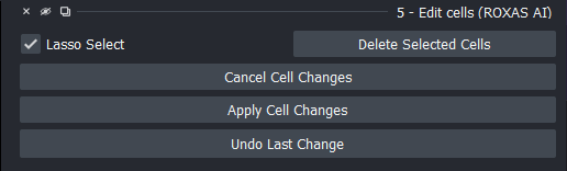
Figure 6: Using lasso selection in vector mode to batch-remove resin canal cells and preparation artifacts.

Step 4: Tree-Ring Editing & Boundary Curation¶

Expand 6 - Edit rings in the Manual Editing group.

Boundary Curation, Nudging & Wedging Rings¶

Fine & Fast Nudging: Select one or more ring boundaries and press Ctrl + Arrow keys (1 px shift) or Ctrl + Shift + Arrow keys (10 px shift) to align boundaries perfectly along the terminal latewood tracheid row.
Adding Missing Rings: Draw a path across the wood cross-section using napari's path tool; ROXAS AI automatically completes the line horizontally to both image margins (\(x=0\) to \(x=\text{width}\)) upon applying changes.
Handling Wedging / Incomplete Rings:
1. Select and copy-paste the existing boundary that shares the common portion of the ring boundary.
2. Enable Lasso Select and draw a lasso loop around the diverging section of the duplicated (topmost) ring.
3. Press Delete or Backspace. ROXAS AI's top-priority lasso logic deletes vertices strictly from the topmost ring, keeping the underlying shared boundary completely intact.
4. Use the path tool to extend and accurately trace the wedging branch.
Re-running AI Ring Segmentation Below Corrected Ring: Select a verified ring boundary and trigger a model re-run to re-segment all rings below that year without disturbing validated boundaries above.
Updating Outermost Calendar Year: Adjust the outermost year in the widget and click Update Year (supports calendar years from -100,000 to 9,999).
Undo (Ctrl + Z): Reverts any drawing, nudging, affine transformation, or deletion (up to 50 undo steps).

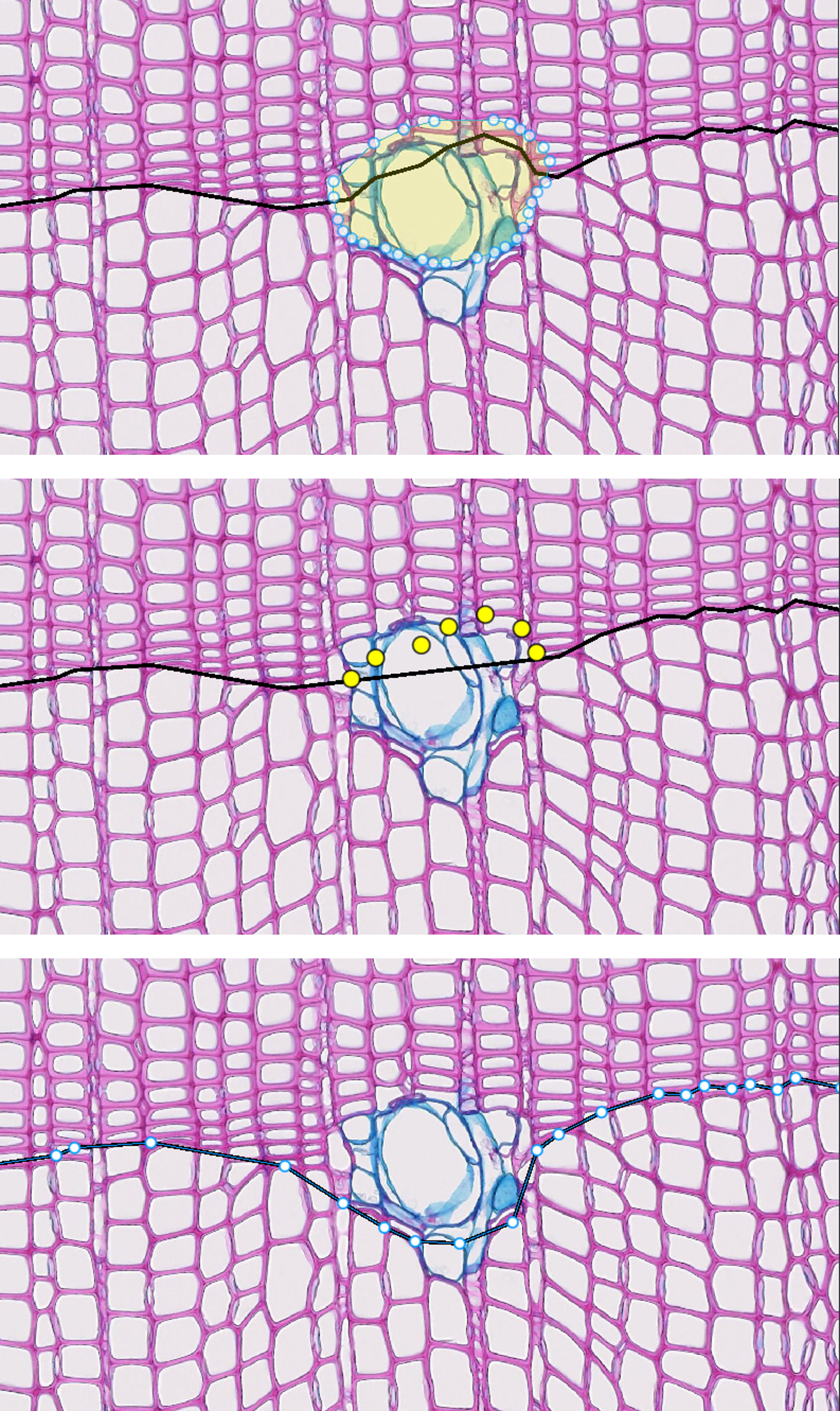
Figure 7: Curating tree-ring boundary polylines in the napari canvas, including vertex dragging, boundary nudging, and wedging ring tracing.

Step 5: Visual Cross-Dating & Ring Synchronization¶

Open Plugins > ROXAS AI > 7 - Visual crossdating to verify ring counts and calendar year assignments against master chronologies.

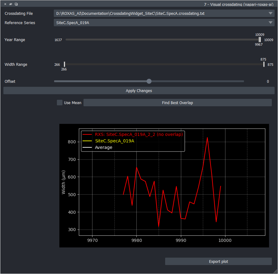
Figure 8: Visual cross-dating plotter showing sample ring widths synchronized against reference series.

Automatic File Discovery & Upward Traversal:
- The plotter searches strictly upwards from the sample folder through parent project directories to auto-discover all available .crossdating.txt files.
Reference Series Selection:
- Select reference series from the dropdown (or use the site composite curve with Use Mean). ROXAS AI automatically prioritizes series names matching the sample stem.
Inspect Standard View (\(\pm 10\) Years):
- The plotter opens centered on the sample series with an overview buffer of \(\pm 10\) years on each side.
Expand Year Range & Offset Slider:
- To explore candidate shifts larger than \(\pm 10\) years, widen the Year Range slider; this automatically expands the bounds of the Offset slider, allowing you to slide the sample across larger time spans.
Auto-Offset Alignment:
- Click Find Best Overlap to let ROXAS AI compute candidate alignments ranked by statistical correlation (\(r\)), Gleichläufigkeit (GLK), and \(t\)-value. Interactive candidate alignment buttons allow instantaneous toggling between suggested shifts.
Confirm Dating & Export Plot:
- Click Apply Changes to update the sample's outermost complete year metadata, shift ring years across .rings and .rings_table.csv, and regenerate <sample>_annotated.jpg.
- Click Export Plot to save a publication-ready <sample>_ReferenceSeries.jpg image (rendered with a standardized 70 px/year aspect ratio) in the sample directory.

Step 6: Saving Verified Annotations¶

Click Save All Layers inside the active editor or open 8 - Save cells & rings editing.

Modified-Layer Tracking: Checks which layers have pending changes (layer.metadata["is_modified"] = True) and saves only modified files to disk:
- .cells.png (8-bit or 16-bit label mask).
- .rings.tif (16-bit TIFF label mask).
- .metadata.json (synchronized metadata record with updated ring counts, outermost year, and timestamps).
Explicit Save Status Notifications: Displays clear feedback: "Saved cells layer.", "Saved rings layer.", "Saved cells and rings layers.", or "No unsaved changes in cells or rings layers.".
Fast Decoupled Saving: Manual layer saving does not redraw the annotated overview image, ensuring saves complete in milliseconds without disk or CPU overhead. The overview image is automatically re-rendered at key workflow checkpoints (AI segmentation, Year updates, Cross-dating application, and Trait measurement).

Figure 9: Saving finalized annotation layers to disk.

Step 7: Anatomical Traits Extraction & Chronology Export¶

In the Manual Editing group, scroll to 9A - Measure cells & rings (individual image).
Check Measure Cells and/or Measure Rings.
(Optional) Click Check Settings to review or customize measurement parameters and quality control thresholds.
Click Measure.
The measurement engine computes anatomical traits via CWT and wall profiling, cleans non-measured edge artefacts, attaches measurements to layer properties for interactive table inspection, and outputs comprehensive semicolon-delimited CSV tables and quality assurance datasets:
- <sample>.cells_table.csv: Individual cell metrics (CID, YEAR, LA, CWTRAD, CWTTAN, CWTALL, RTSR, KH, DH).
- <sample>.rings_table.csv: Ring summary metrics (YEAR, MRW, CNO, MLA, CD, CWTALL, RWD, RCTA).
- <sample>.cwt.json: Exported CWT quality assurance dataset containing circle coordinates, wall thickness values, inclusion/exclusion flags, and exclusion reasons.
- [<sample>] CWT Circles Shapes Layer: Interactive viewer layer with hover tooltips displaying Cell ID, sector, thickness (\(\mu\text{m}\)), status, and exclusion reason for visual QA inspection.
- <sample>_annotated.jpg: Automatically regenerated and saved with synchronized ring boundaries, calendar years, and cell lumen highlights matching the final measurements.
- <sample>_ReferenceSeries.jpg: Saved in the sample directory when cross-dating was performed and applied.

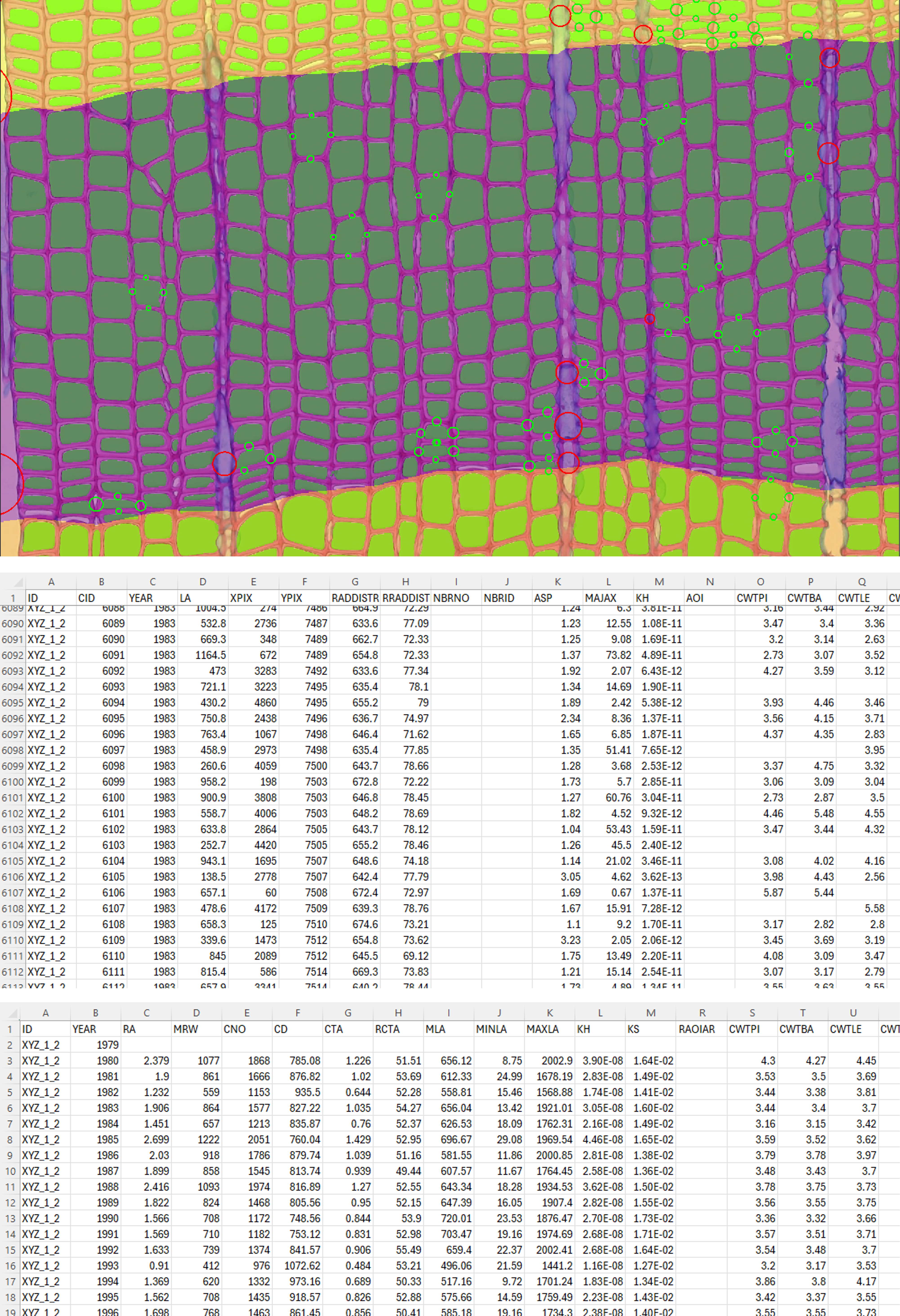
A: Measurement ControlsB: In-Viewer CWT QA Layer

Figure 10: Single sample trait extraction and quality assurance: (A) Measurement control panel and (B) In-viewer CWT circles overlay with hover tooltips alongside extracted feature tables.

3. Production Workflow: Batch Processing Multi-Sample Studies¶

When analyzing dozens or hundreds of wood sections, ROXAS AI provides an automated batch processing pipeline to maximize throughput while guaranteeing complete file synchronization across all sample folders.

flowchart TD
    B1["1. Batch Preparation (Widget 1 / Ctrl+Shift+B)"] --> B2["2. Batch AI Detection (Widget 3B)"]
    B2 --> B3["3. Targeted Quality Control (Group Ctrl+Shift+M)"]
    B3 --> B4["4. Batch Measure & Synchronize (Widget 9B)"]

Step 1: Batch Preparation & Standardization¶

Organize raw cross-section scans into your project folder.
Launch napari-roxas and press Ctrl + Shift + B to open the Batch Operations Group.
In 1 - Prepare project images for analysis:
- Select your project directory (or use 0 - Define project directory).
- Batch-assign physical spatial resolution (\(\text{px}/\mu\text{m}\)), sample type, and geometry across all matching images.
- Import reference cross-dating chronologies if available.
Click Prepare Images to standardize filenames (<sample>.scan.<ext>) and initialize <sample>.metadata.json across the entire dataset.

Step 2: Batch Cell & Ring Segmentation¶

In the same batch container, scroll to 3B - Batch detect cells & rings.
Real-Time Dynamic Sync: The widget automatically listens to the project directory so all newly prepared samples appear immediately in the file list.
Select your deep-learning models (linear_cells_model and LinearRingModel_v3_iterative.pt).
Click Run Batch Segmentation.
The multi-threaded background queue processes each sample sequentially, creating <sample>.cells.png and <sample>.rings.tif masks without loading full-resolution images into memory.

Step 3: Targeted Quality Control¶

Press Ctrl + Shift + M to switch to the Manual Editing Group.
In 2/4 - Load image(s), iterate through samples to inspect automated predictions.
Perform targeted curation as needed:
- 5 - Edit cells: Use Vector Lasso Select (Delete) to batch-remove resin canal cells or preparation defects.
- 6 - Edit rings: Nudge boundaries (Ctrl+Arrows), add missing rings, or curate wedging rings.
- 7 - Visual cross-dating: Verify ring counts and synchronize calendar dating against master chronologies.
Click Save All Layers (or use 8 - Save cells & rings editing) to persist curated layers.

Step 4: Automated Batch Measurement & File Synchronization¶

Press Ctrl + Shift + B to return to the Batch Operations Group.
In 9B - Batch measure & update:
- Check Measure Cells and Measure Rings.
- Linked Operations Locking: Notice that Update Annotated image and Update Crossdating Reference Files are automatically locked ON whenever measurements are active. This guarantees that all numerical CSV tables, CWT JSON files (.cwt.json), annotated overview images (_annotated.jpg), and reference cross-dating plots (_ReferenceSeries.jpg) remain 100% consistent and synchronized across every sample folder in the project.
- Reference Plot Auto-Generation: ROXAS AI automatically searches upwards through the directory tree for cross-dating files and matches sample stems to reference chronologies (or uses the validated reference_series in metadata).
Click Measure & Update.
The batch engine executes across all samples, writing .cells_table.csv, .rings_table.csv, .cwt.json, _annotated.jpg, and _ReferenceSeries.jpg directly to each sample folder.

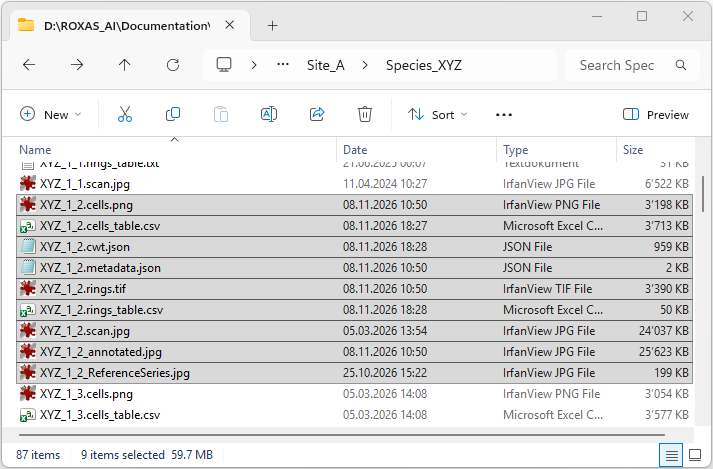
Figure 11: Standardized sample folder file hierarchy generated after batch processing (.cells.png, .rings.tif, .cells_table.csv, .rings_table.csv, .cwt.json, _annotated.jpg, and _ReferenceSeries.jpg).